######### ggraph version 2
require(bipartite)
require(igraph)
require(ggplot2)
require(NetIndices)
# gggraph, version 2
# g = an igraph graph object, a matrix, or data frame
# vplace = type of vertex placement assignment, one of rnorm, runif, etc.
# method = one of 'df' for data frame, "mat' for matrix or "igraph" for an igraph graph object
# trophic = TRUE or FALSE for using Netindices function TrophInd to determine trophic level (y value in graph)
# trophinames = columns in matrix or dataframe to use for calculating trophic level
# import = named or refereced by col# columns of matrix or dataframe to use for import argument of TrophInd
# export = named or refereced by col# columns of matrix or dataframe to use for export argument of TrophInd
# dead = named or refereced by col# columns of matrix or dataframe to use for dead argument of TrophInd
gggraph <- function(g, vplace = rnorm, method, trophic = "FALSE",
trophinames, import, export)
{
degreex <- function(x) {
degreecol <- apply(x, 2, function(y) length(y[y>0]))
degreerow <- apply(x, 1, function(y) length(y[y>0]))
degrees <- sort(c(degreecol, degreerow))
df <- data.frame(degrees, x = seq(1, length(degrees), 1))
df$value <- rownames(df)
df
}
# require igraph
if(!require(igraph)) stop("must first install 'igraph' package.")
# require ggplot2
if(!require(ggplot2)) stop("must first install 'ggplot2' package.")
if(method=="df"){
if(class(g)=="matrix"){ g <- as.data.frame(g) }
if(class(g)!="data.frame") stop("object must be of class 'data.frame.'")
if(trophic=="FALSE"){
# data preparation from adjacency matrix
temp <- data.frame(expand.grid(dimnames(g))[1:2], as.vector(as.matrix(g)))
temp <- temp[(temp[, 3] > 0) & !is.na(temp[, 3]), ]
temp <- temp[sort.list(temp[, 1]), ]
g_df <- data.frame(rows = temp[, 1], cols = temp[, 2], freqint = temp[, 3])
g_df$id <- 1:length(g_df[,1])
g_df <- data.frame(id=g_df[,4], rows=g_df[,1], cols=g_df[,2], freqint=g_df[,3])
g_df <- melt(g_df, id=c(1,4))
xy_s <- data.frame(degreex(g), y = rnorm(length(unique(g_df$value))))
g_df_2 <- merge(g_df, xy_s, by = "value")
} else if(trophic=="TRUE") {
# require NetIndices
if(!require(NetIndices)) stop("must first install 'NetIndices' package.")
# data preparation from adjacency matrix
temp <- data.frame(expand.grid(dimnames(g[-trophinames, -trophinames]))[1:2],
as.vector(as.matrix(g[-trophinames, -trophinames])))
temp <- temp[(temp[, 3] > 0) & !is.na(temp[, 3]), ]
temp <- temp[sort.list(temp[, 1]), ]
g_df <- data.frame(rows = temp[, 1], cols = temp[, 2], freqint = temp[, 3])
g_df$id <- 1:length(g_df[,1])
g_df <- data.frame(id=g_df[,4], rows=g_df[,1],
cols=g_df[,2], freqint=g_df[,3])
g_df <- melt(g_df, id=c(1,4))
xy_s <- data.frame(value = unique(g_df$value),
x = rnorm(length(unique(g_df$value))),
y = TrophInd(g, Import=import, Export=export)[,1])
g_df_2 <- merge(g_df, xy_s, by = "value")
}
# plotting
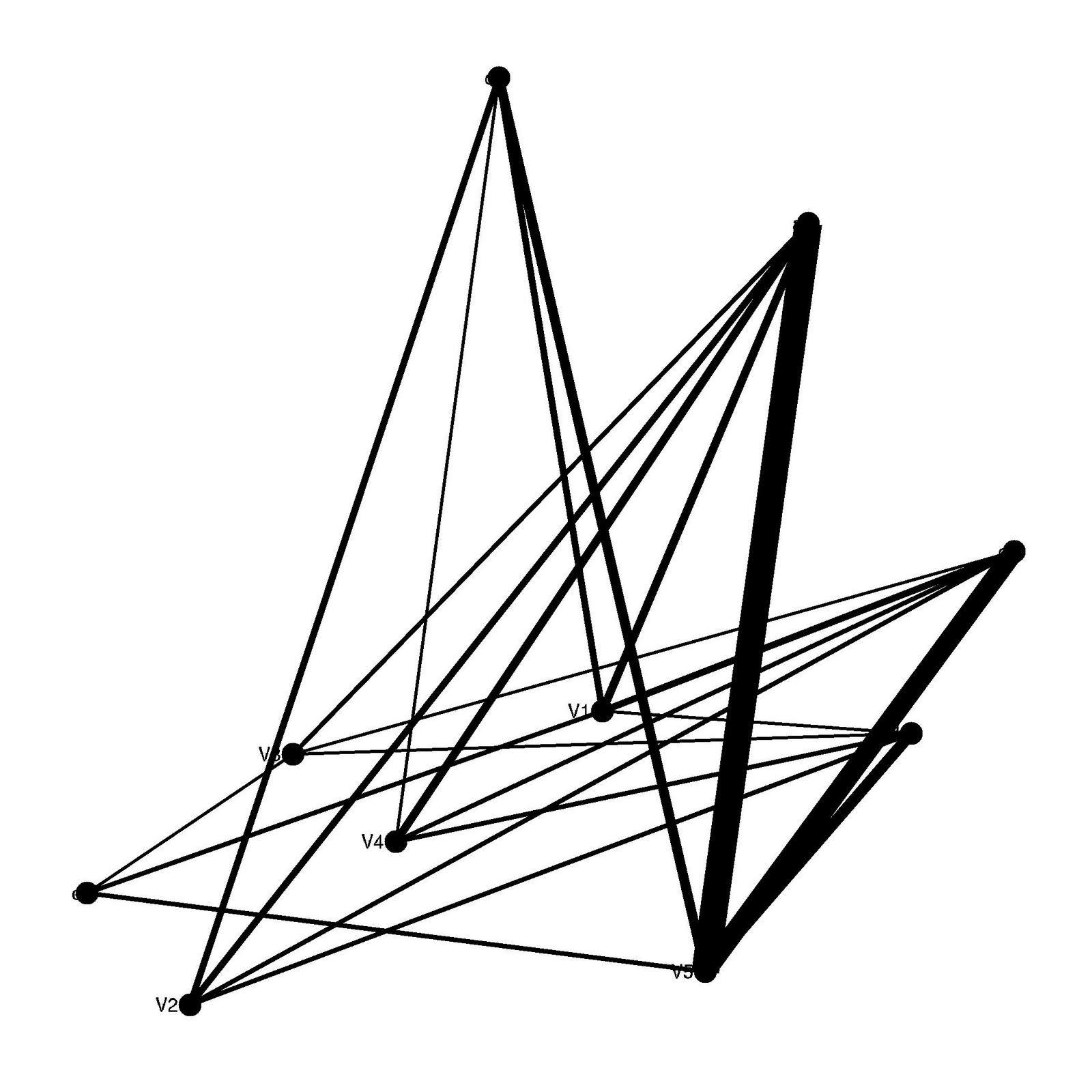
p <- ggplot(g_df_2, aes(x, y)) +
geom_point(size = 5) +
geom_line(aes(size = freqint, group = id)) +
geom_text(size = 3, hjust = 1.5, aes(label = value)) +
theme_bw() +
opts(panel.grid.major=theme_blank(),
panel.grid.minor=theme_blank(),
axis.text.x=theme_blank(),
axis.text.y=theme_blank(),
axis.title.x=theme_blank(),
axis.title.y=theme_blank(),
axis.ticks=theme_blank(),
panel.border=theme_blank(),
legend.position="none")
p # return graph
} else if(method=="igraph") {
if(class(g)!="igraph") stop("object must be of class 'igraph.'")
# data preparation from igraph object
g <- get.edgelist(g)
g_df <- as.data.frame(g_)
g_df$id <- 1:length(g_df[,1])
g_df <- melt(g_df, id=3)
xy_s <- data.frame(value = unique(g_df$value),
x = vplace(length(unique(g_df$value))),
y = vplace(length(unique(g_df$value))))
g_df2 <- merge(g_df, xy_s, by = "value")
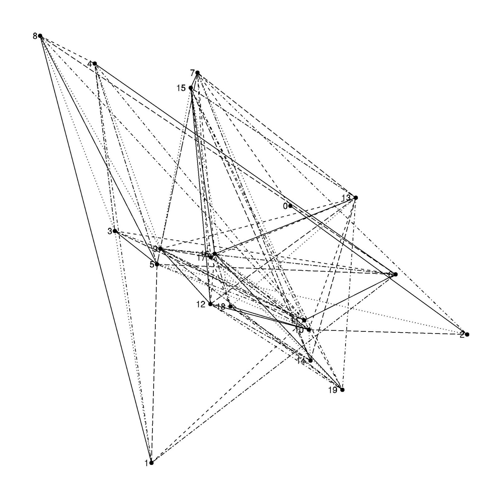
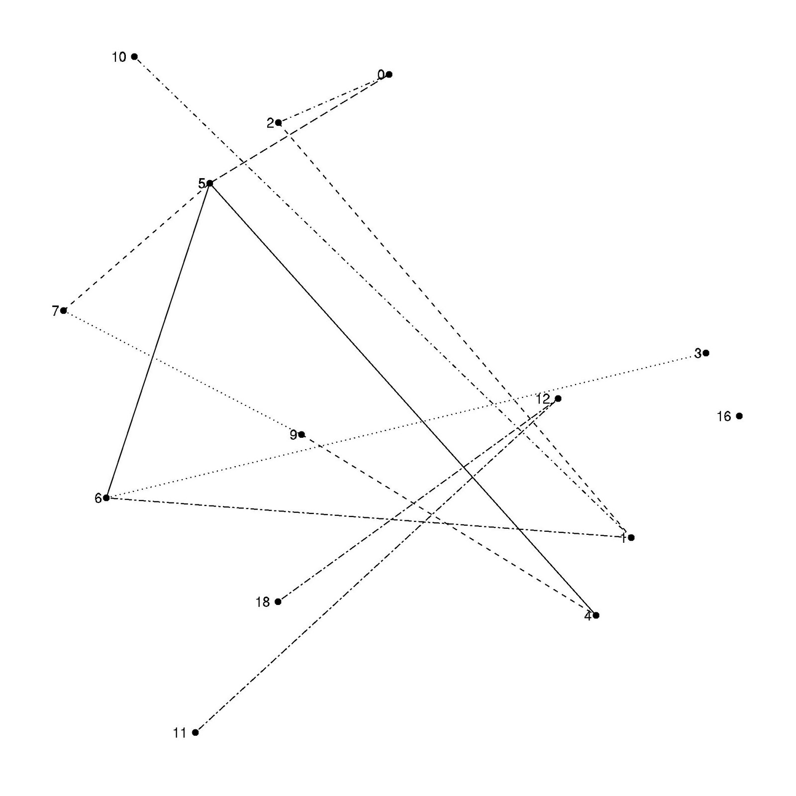
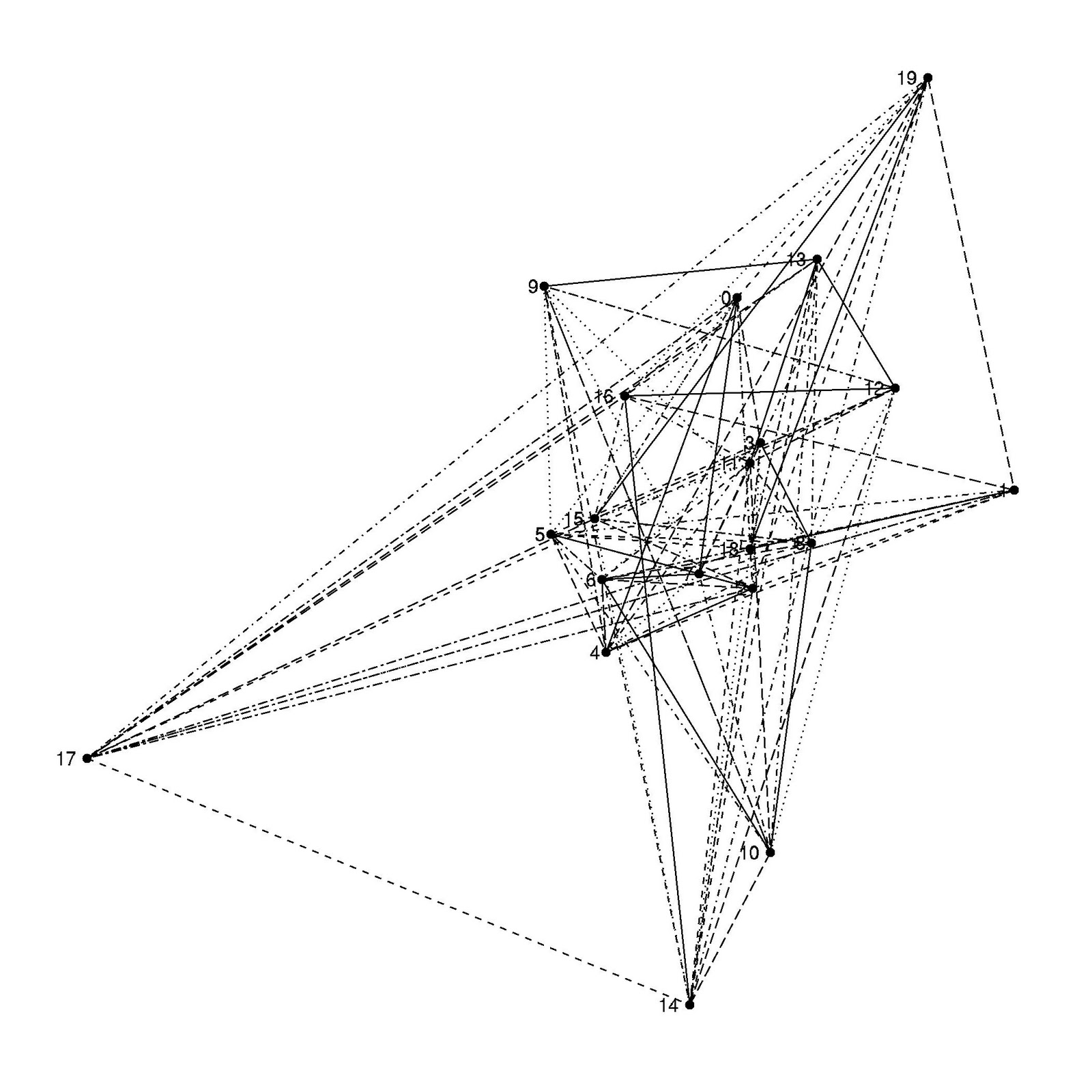
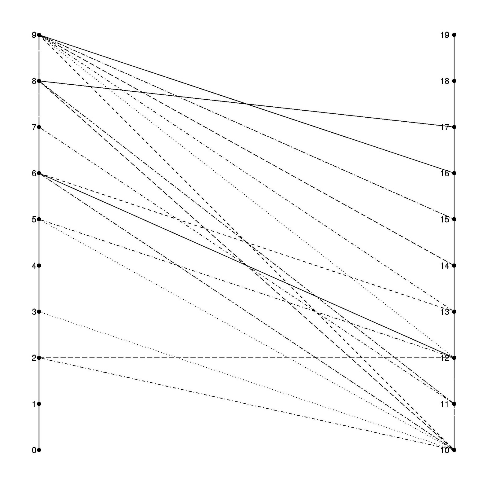
# plotting
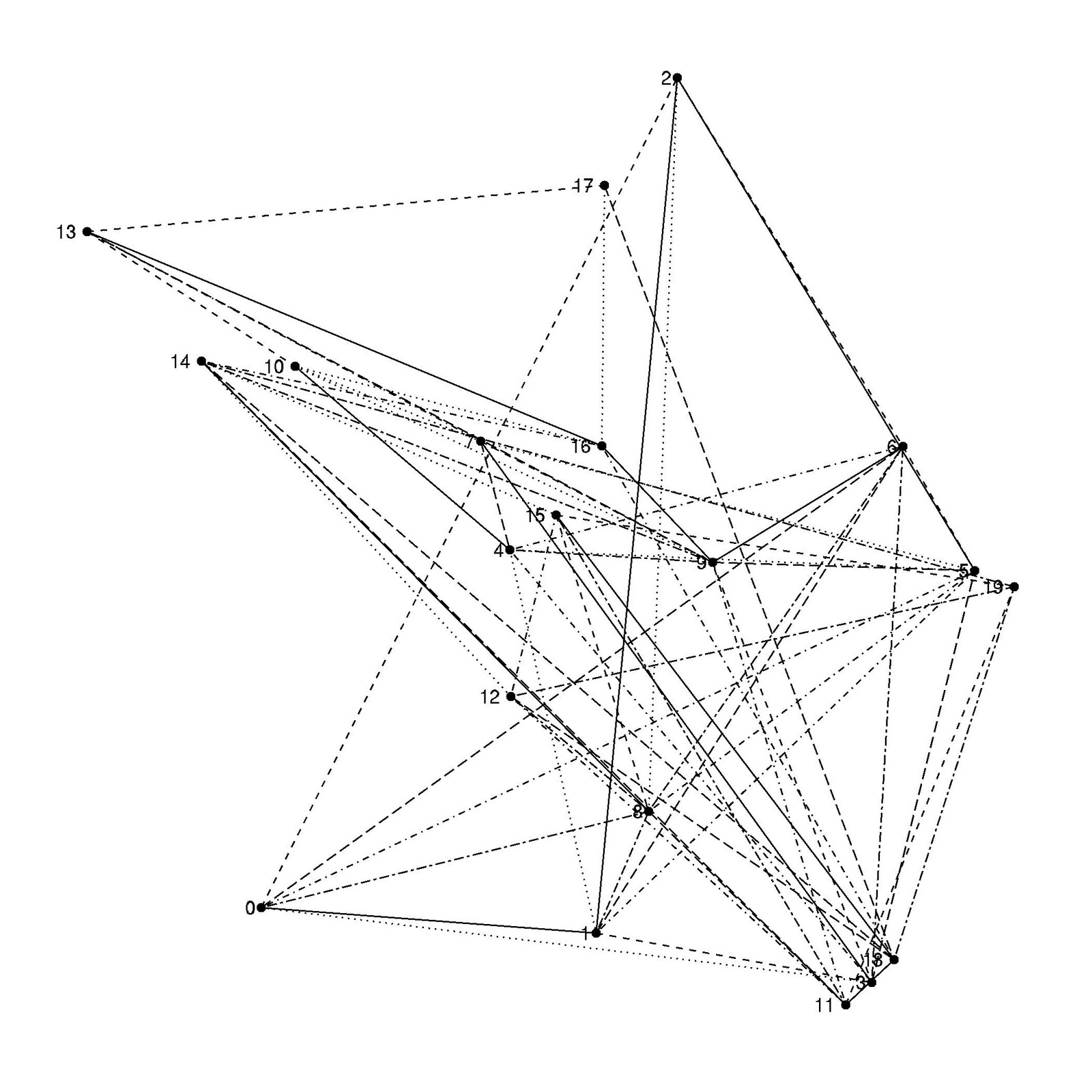
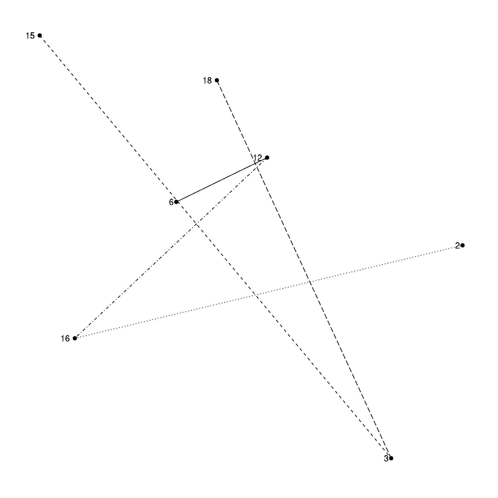
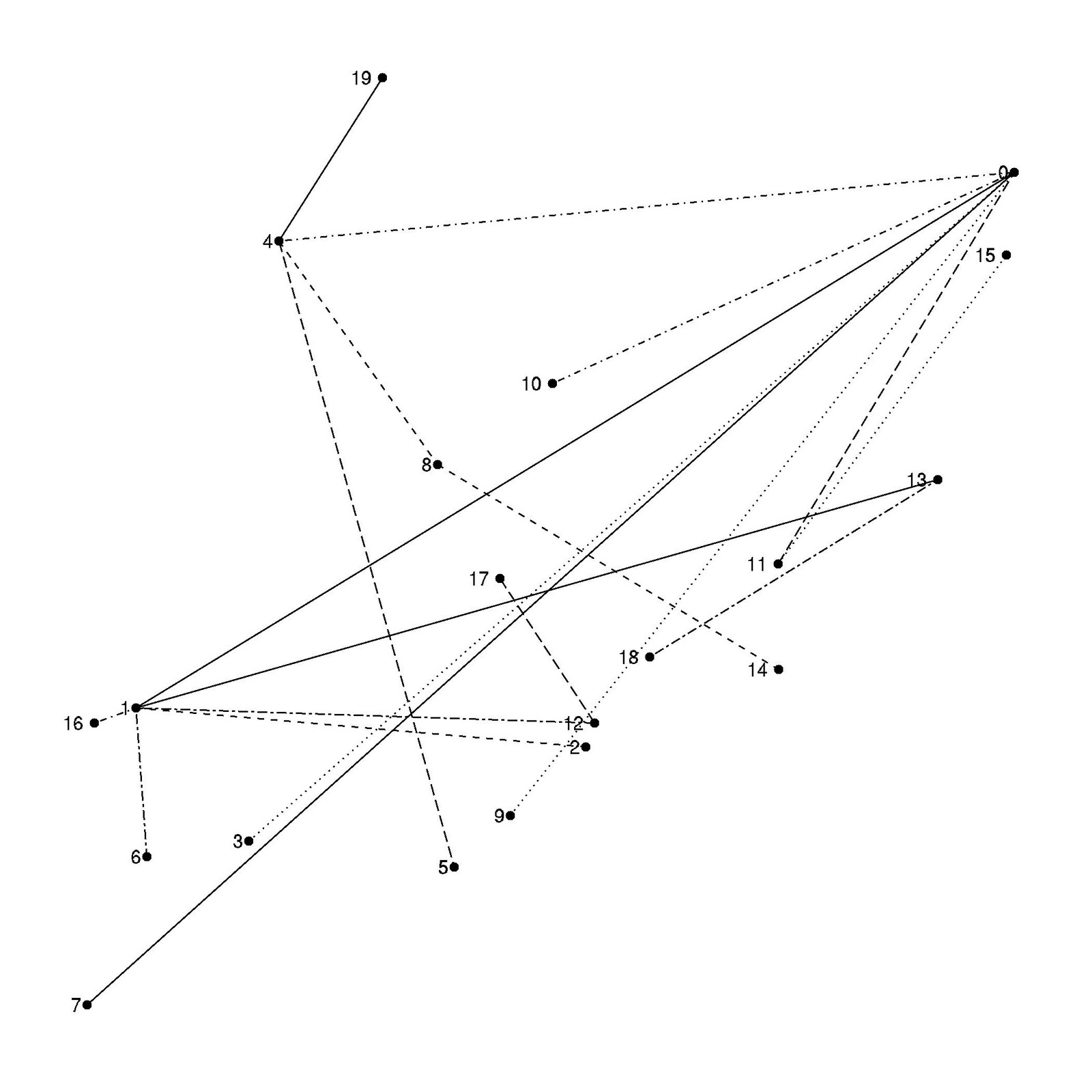
p <- ggplot(g_df2, aes(x, y)) +
geom_point(size = 2) +
geom_line(size = 0.3, aes(group = id, linetype = id)) +
geom_text(size = 3, hjust = 1.5, aes(label = value)) +
theme_bw() +
opts(panel.grid.major=theme_blank(),
panel.grid.minor=theme_blank(),
axis.text.x=theme_blank(),
axis.text.y=theme_blank(),
axis.title.x=theme_blank(),
axis.title.y=theme_blank(),
axis.ticks=theme_blank(),
panel.border=theme_blank(),
legend.position="none")
p # return graph
} else
stop(paste("do not recognize method = \"",method,"\";
methods are \"df\" and \"igraph\"",sep=""))
}