Processing nested lists

Author  Scott Chamberlain

So perhaps you have all figured this out already, but I was excited to figure out how to finally neatly get all the data frames, lists, vectors, etc. out of a nested list. It is as easy as nesting calls to the apply family of functions, in the case below, using plyr's apply like functions. Take this example:


# Nested lists code, an example
# Make a nested list
mylist <- list()
mylist <- list()
for(i in 1:5) {
for(j in 1:5) {
mylist[[j]] <- i*j
}
mylist
[[i]] <- mylist
}
 
# return values from first part of list
laply(mylist[[1]], identity)
[1] 1 2 3 4 5
 
# return all values
laply(mylist
, function(x) laply(x, identity))
1 2 3 4 5
[1,] 1 2 3 4 5
[2,] 2 4 6 8 10
[3,] 3 6 9 12 15
[4,] 4 8 12 16 20
[5,] 5 10 15 20 25
 
# perform some function, in this case sqrt of each value
laply(mylist_, function(x) laply(x, function(x) sqrt(x)))
  
1 2 3 4 5
[1,] 1.000000 1.414214 1.732051 2.000000 2.236068
[2,] 1.414214 2.000000 2.449490 2.828427 3.162278
[3,] 1.732051 2.449490 3.000000 3.464102 3.872983
[4,] 2.000000 2.828427 3.464102 4.000000 4.472136
[5,] 2.236068 3.162278 3.872983 4.472136 5.000000


Created by Pretty R at inside-R.org

Posted in  R

Author  Scott Chamberlain

Running Phylip's contrast application for trait pairs from R

Author  Scott Chamberlain

Here is some code to run Phylip's contrast application from R and get the output within R to easily manipulate yourself. Importantly, the code is written specifically for trait pairs only as the regular expression work in the code specifically grabs data from contast results when only two traits are input. You could easily change the code to do N traits. Note that the p-value calculated for the chi-square statistic is not output from contrast, but is calculated within the function 'PhylipWithinSpContr'. In the code below there are two functions that make a lot of busy work easier: 'WritePhylip' and 'PhylipWithinSpContr'. The first function is nice because the formatting required for data input to Phylip programs is so, well, awkward  - and this function does it for you. The second function runs contrast and retrieves the output data. The example data set I produce in the code below has multiple individuals per species, so that contrasts are calculated taking into account within species variation. Get Phylip's contrast documentation here.

Note that the data input format allows only 10 characters for the species name, so I suggest if your species names are longer than 10 characters use the function abbreviate, for example, to shorten all names to no longer than 10 characters. Also, within the function WritePhylip I concatenate species names and their number of individuals per species leaving plenty of space.

Also, mess around with the options in the "system" call to get what you want. For example, I used "R", "W" and "Y", meaning replace old outfile (R), then turn on within species analyses (W), then accept all options (Y). E..g, if you don't have an old outfile, then you obviously don't need to replace the old file with the "R" command.

(p.s. I have not tried this on a windows machine).


Here is example output:


> datout
names2 dat...1. dat...2.
1 VarAIn_VarAest 0.000110 -0.000017
2 VarAIn_VarAest -0.000017 0.000155
3 VarAIn_VarEest 0.790783 -0.063097
4 VarAIn_VarEest -0.063097 0.981216
5 VarAIn_VarAreg 1.000000 -0.107200
6 VarAIn_VarAreg -0.151800 1.000000
7 VarAIn_VarAcorr 1.000000 -0.127600
8 VarAIn_VarAcorr -0.127600 1.000000
9 VarAIn_VarEreg 1.000000 -0.064300
10 VarAIn_VarEreg -0.079800 1.000000
11 VarAIn_VarEcorr 1.000000 -0.071600
12 VarAIn_VarEcorr -0.071600 1.000000
13 VarAOut_VarEest 0.790734 -0.063104
14 VarAOut_VarEest -0.063104 0.981169
15 VarAOut_VarEreg 1.000000 -0.064300
16 VarAOut_VarEreg -0.079800 1.000000
17 VarAOut_VarEcorr 1.000000 -0.071600
18 VarAOut_VarEcorr -0.071600 1.000000
19 logL_withvar_df -68.779770 6.000000
20 logL_withoutvar_df -68.771450 3.000000
21 chisq_df -0.016640 3.000000
22 chisq_p 1.000000 -999.000000
Posted in  Phylogenetics R

Author  Scott Chamberlain

Phylometa from R: Randomization via Tip Shuffle

Author  Scott Chamberlain

---UPDATE: I am now using code formatting from gist.github, so I replaced the old prettyR code (sorry guys). The github way is much easier and prettier. I hope readers like the change.


I wrote earlier about some code I wrote for running Phylometa (software to do phylogenetic meta-analysis) from R.

I have been concerned about what exactly is the right penalty for including phylogeny in a meta-analysis. E.g.: AIC is calculated from Q in Phylometa, and Q increases with tree size.

So, I wrote some code to shuffle the tips of your tree N number of times, run Phylometa, and extract just the "Phylogenetic MA" part of the output. So, we compare the observed output (without tip shuffling) to the distribution of the tip shuffled output, and we can calculate a P-value from that. The code I wrote simply extracts the pooled effect size for fixed and also random-effects models. But you could change the code to extract whatever you like for the randomization.

I think the point of this code is not to estimate your pooled effects, etc., but may be an alternative way to compare traditional to phylogenetic MA where hopefully simply incorporating a tree is not penalizing the meta-analysis so much that you will always accept the traditional MA as better.

Get the code here, and also below. Get the example tree file and data file, named "phylogeny.txt" and "metadata_2g.txt", respectively below (or use your own data!). You need the file "phylometa_fxn.r" from my website, get here, but just call it using source as seen below.


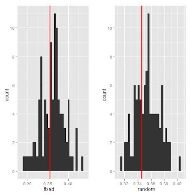
As you can see, the observed values fall well within the distribution of values obtained from shuffling tips.  P-values were 0.64 and 0.68 for fixed- and random-effects MA's, respectively. This suggests, to me at least, that the traditional (distribution of tip shuffled analyses, the histograms below) and phylogenetic (red lines) MA's are not different. The way I would use this is as an additional analysis to the actual Phylometa output.

Posted in  meta-analysis Methods Evolution Phylogenetics R

Author  Scott Chamberlain

RStudio Beta 2 is Out!

Author  Scott Chamberlain

RStudio Beta 2 (v0.93) « RStudio Blog


A new beta version of RStudio is out!

Posted in 

Author  Scott Chamberlain

Adjust branch lengths with node ages: comparison of two methods

Author  Scott Chamberlain

Here is an approach for comparing two methods of adjusting branch lengths on trees: bladj in the program Phylocom and a fxn written by Gene Hunt at the Smithsonian.

Get the code and example files (tree and node ages) here
Get phylocom here: http://www.phylodiversity.net/phylocom/

Gene Hunt's method has many options you can mess with, including setting tip ages (not available in bladj), setting node ages, and minimum branch length imposed. You will notice that Gene's method may be not the appropriate if you only have extant taxa.

The function AdjBrLens uses as input a newick tree file and a text file of node ages, and uses functions you can simply run by "source" the R file bladjing_twomethods.R file from here.

Note that blad does not like numbers for node names, so you have to put a character in front of a number of just character names for nodes.


# This is where the work happens... 
# Directory below needs to have at least three items:
# 1. phylocom executable for windows or mac
# 2. tree newick file
# 3. node ages file as required by phylocom, see their manual
# Output: trees_out is a list of three trees, the original, bladj, and Gene Hunt's method
# Also, within the function all three trees are written to file as PDFs
setwd("/Mac/R_stuff/Blog_etc/Bladjing") # set working directory
source("bladjing_twomethods.R") # run functions from source file
trees_out <- AdjBrLens("tree.txt", "nodeages.txt")
 
# plot trees of three methods together,
# with nodes with age estimates labeled
jpeg("threeplots.jpeg", quality=100)
layout(matrix(1:3, 1, 3))
plot(trees_out[[1]])
nodelabels(trees_out[[1]]$node.label, cex = 0.6)
title("original tree")
plot(trees_out[[2]])
nodelabels(trees_out[[2]]$node.label, cex = 0.6)
title("bladj method")
plot(trees_out[[3]])
nodelabels(trees_out[[3]]$node.label, cex = 0.6)
title("gene hunt method, scalePhylo")
dev.off()
Created by Pretty R at inside-R.org


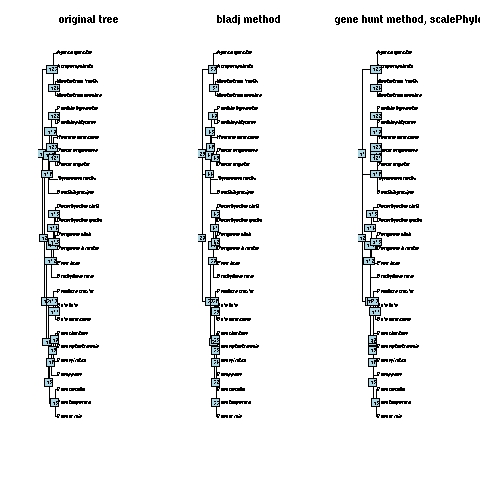
It is sort of hard to see the differences in the branch length changes here, but the individual output trees will reveal the differences better.

Posted in  phylocom Methods Evolution Phylogenetics R

Author  Scott Chamberlain

Fork me on GitHub